最適化手法のテストに利用される有名なベンチマーク関数を一覧にしました。
目次
・最適化とその難しさ
・ベンチマーク関数20種
# Ackley function
# Bukin function N.6
# Booth function
# Beale function
# Drop-Wave function
# Easom function
# Eggholder function
# Goldstein–Price function
# Himmelblau’s function
# Lévi function N.13
# Matyas function
# McCormick function
# Perm function
# Rastrigin function
# Rosenbrock function (banana function)
# Sphere function
# Shubert function
# Styblinski-Tang function
# Three-hump camel function
# Zakharov function
・リンク
最適化とその難しさ
目的関数に対して(多くの場合、幾つかの制約条件下で)値を最大または最小にするような変数の値を求めることを最適化と呼びます。
最適化の難しさは目的関数の形状によって大きく異なります。下の図は “Nature-Inspired Algorithms for Optimisation” という書籍の第1章 “Why Is Optimization Difficult?”「なぜ最適化は難しいのか?」から引いた図で、1.aから1.hまで様々なバリエーションの目的関数のグラフが描かれています。
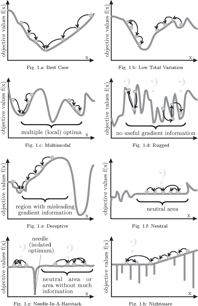
図.目的関数の種類と最適化
(”Nature-Inspired Algorithms for Optimisation“, Chapter 1 “Why Is Optimization Difficult?” より引用)
関数の形状が下の方のタイプに近いほど最適化は難しくなります。1.aは大域的最適解が一つしか存在しないので最適化は容易ですが、1.gや1.hのように鋭いピーク状の極小点が存在する場合は最適化が著しく困難になります。
ベンチマーク関数20種
最適化手法を評価する際に、ベンチマークとして用いられる関数が幾つか知られています。ここでは20種類の主要なベンチマーク関数について、2変数の場合の図とともに紹介します。
Ackley function
# Ackley function
Z = -20*np.exp(-0.2*np.sqrt(0.5*(X**2+Y**2)))-np.exp(0.5*(np.cos(2*np.pi*X)+np.cos(2*np.pi*Y)))+np.e+20
$$\small f(\mathbf{x})=-a \exp \left(-b \sqrt{\frac{1}{d} \sum_{i=1}^{d} x_{i}^{2}}\,\right)-\exp \left(\frac{1}{d} \sum_{i=1}^{d} \cos \left(c x_{i}\right)\right)+a+\exp (1)$$点 $\mathbf{x}^{*}=(0, \ldots, 0)$ で大域的最適解 $f\left(\mathbf{x}^{*}\right)=0$ をとる多峰性関数。
パラメータの推奨値:$a = 20$、$b = 0.2$、$c = 2\pi$($d$は次元数)
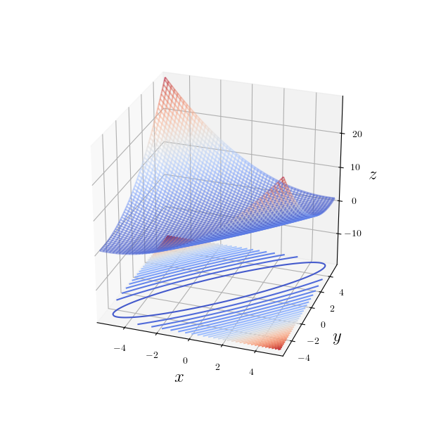
Bukin function N.6
# Bukin function N.6
Z = 100 * np.sqrt(abs(Y - 0.01*X**2)) + 0.01*abs(X + 10)
$$f(\mathbf{x})=100 \sqrt{\left|x_{2}-0.01 x_{1}^{2}\right|}+0.01\left|x_{1}+10\right|$$点 $\mathbf{x}^{*}=(-10,\, 1)$ で大域的最適解 $f\left(\mathbf{x}^{*}\right)=0$ をとる多峰性関数。微分可能でない点が多く、収束のシビアな関数として知られる。
Booth function
# Booth function
Z = (X + 2*Y - 7)**2 + (2*X + Y - 5)**2
$$f(\mathbf{x})=\left(x_{1}+2 x_{2}-7\right)^{2}+\left(2 x_{1}+x_{2}-5\right)^{2}$$点 $\mathbf{x}^{*}=(1,\, 3)$ で大域的最適解 $f\left(\mathbf{x}^{*}\right)=0$ をとる単峰性関数。
Beale function
# Beale function
Z = (1.5 - X + X*Y)**2 + (2.25 - X + X * (Y**2))**2 + (2.625 - X + X * (Y**3))**2
$$\small \begin{align} f(\mathbf{x})=&\left(1.5-x_{1}+x_{1} x_{2}\right)^{2} \\ &+\left(2.25-x_{1}+x_{1} x_{2}^{2}\right)^{2}+\left(2.625-x_{1}+x_{1} x_{2}^{3}\right)^{2} \end{align}$$点 $\mathbf{x}^{*}=(3,\, 0.5)$ で大域的最適解 $f\left(\mathbf{x}^{*}\right)=0$ をとる多峰性関数。ただし$0$は最小値ではない。例えば $\displaystyle \lim_{x_1 \to \infty}f(\mathbf{x})$ は $x_2=1$ の極近傍で負の値をとる。$(0,\, 1)$などが停留点として得られる場合があるが極小点ではない。$f(0,\,x_2)=f(x_1,\,1)=14.203125$が成り立つ。
Drop-Wave function
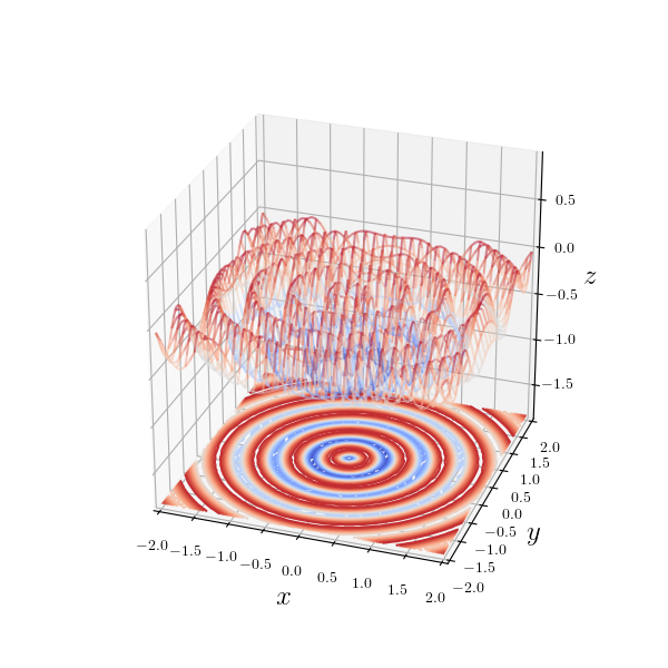
# Drop-Wave function
Z = -(1 + np.cos(12 * np.sqrt(X**2 + Y**2)))/((0.5 * (X**2 + Y**2)) + 2)
$$f(\mathbf{x})=-\dfrac{1+\cos \left(12 \sqrt{x_{1}^{2}+x_{2}^{2}}\right)}{0.5\left(x_{1}^{2}+x_{2}^{2}\right)+2}$$点 $\mathbf{x}^{*}=(0,\, 0)$ で大域的最適解 $f\left(\mathbf{x}^{*}\right)=0$ をとる多峰性関数。
Easom function
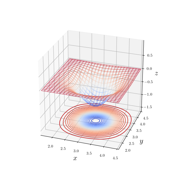
# Easom function
Z = -np.cos(X)*np.cos(Y)*np.exp(-Y**2 + 2*np.pi*Y - X**2 + 2*np.pi*X - 2*np.pi**2)
$$\small f(\mathbf{x})=-\cos \left(x_{1}\right) \cos \left(x_{2}\right) \exp \left(-\left(x_{1}-\pi\right)^{2}-\left(x_{2}-\pi\right)^{2}\right)$$点 $\mathbf{x}^{*}=(\pi,\, \pi)$ で大域的最適解 $f\left(\mathbf{x}^{*}\right)=-1$ をとる単峰性関数。極小点から遠い位置では勾配がほとんど消失する。
Eggholder function
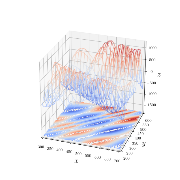
# Easom function
Z = -np.cos(X)*np.cos(Y)*np.exp(-Y**2 + 2*np.pi*Y - X**2 + 2*np.pi*X - 2*np.pi**2)
$$\begin{align} f(\mathbf{x})=&-\left(x_{2}+47\right) \sin \left(\sqrt{ \left| x_{2}+\dfrac{x_{1}}{2}+47\right|} \,\right) \\ &-x_{1} \sin \left(\sqrt{\left|x_{1}-\left(x_{2}+47\right)\right|}\,\right) \end{align}$$点 $\mathbf{x}^{*}=(512,\, 404.2319…\pi)$ で大域的最適解 $f\left(\mathbf{x}^{*}\right)=-959.6407…$ をとる多峰性関数。”Eggholder” の名の通り局所最適解が無数に存在し、大域的最適解の探索が困難な関数の一つ。
Goldstein–Price function
# Goldstein–Price function
f1 = (1+(X+Y+1)**2*(19-14*X+3*X**2-14*Y+6*X*Y+3*Y**2))
f2 = (30+(2*X-3*Y)**2*(18-32*X+12*X**2+48*Y-36*X*Y+27*Y**2))
Z = f1 * f2
$$\small \begin{aligned}
f(\mathbf{x})=&\left[1+\left(x_{1}+x_{2}+1\right)^{2}\left(19-14 x_{1}+3 x_{1}^{2}-14 x_{2}+6 x_{1} x_{2}+3 x_{2}^{2}\right)\right] \\
& \times\left[30+\left(2 x_{1}-3 x_{2}\right)^{2}\left(18-32 x_{1}+12 x_{1}^{2}+48 x_{2}-36 x_{1} x_{2}+27 x_{2}^{2}\right)\right]
\end{aligned}$$点 $\mathbf{x}^{*}=(0,\, -1)$ で大域的最適解 $f\left(\mathbf{x}^{*}\right)=3$ をとる多峰性関数。$(-0.6,\,-0.4)$、$(1.2,\,0.8)$、$(1.8,\,0.2)$で局所最適解をもつ。
Himmelblau’s function
# Himmelblau's function
Z = (X**2 + Y -11)**2 + (X + Y**2 - 7)**2
$$f(\mathbf{x})=(x_1^{2}+x_2-11)^{2}+(x_1+x_2^{2}-7)^{2}$$点 $\mathbf{x}^{*}=(3.0,\, 2.0)$、$(-2.805…,\, 3.131…)$、$(-3.779…,\, -3.283…)$、$(3.584…,\, -1.848…)$ で大域的最適解 $f\left(\mathbf{x}^{*}\right)=0$ をとる多峰性関数。「【最適化問題の基礎】ニュートン法で停留点を探す(鞍点と固有値の関係)」の記事で取り扱っている。
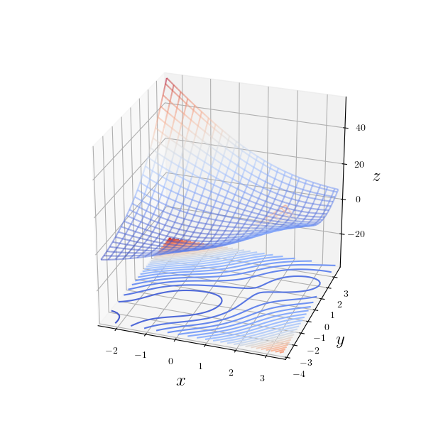
Lévi function N.13
# Lévi function N.13
Z = np.sin(3*np.pi*X)**2 + (X - 1)**2 * (1 + np.sin(3*np.pi*Y)**2) + (Y - 1)**2 * (1 + np.sin(2*np.pi*Y)**2)
$$\begin{align} f(\mathbf{x})=&\sin ^{2}\left(3 \pi x_{1}\right)+\left(x_{1}-1\right)^{2}\left[1+\sin ^{2}\left(3 \pi x_{2}\right)\right] \\ &+\left(x_{2}-1\right)^{2}\left[1+\sin ^{2}\left(2 \pi x_{2}\right)\right] \end{align}$$点 $\mathbf{x}^{*}=(1,\, 1)$ で大域的最適解 $f\left(\mathbf{x}^{*}\right)=0$ をとる多峰性関数。全体がすり鉢状になっており、多数の$x$軸に平行な谷間の中に局所最適解が存在している。
Matyas function
# Matyas function
Z = 0.26 * (X**2 + Y**2) - 0.48 * X * Y
$$f(\mathbf{x})=0.26\left(x_{1}^{2}+x_{2}^{2}\right)-0.48 x_{1} x_{2}$$点 $\mathbf{x}^{*}=(0,\, 0)$ で大域的最適解 $f\left(\mathbf{x}^{*}\right)=0$ をとる単峰性関数。
McCormick function
# McCormick function
Z = np.sin(X + Y) + (X - Y)**2 - 1.5*X + 2.5*Y + 1
$$f(\mathbf{x})=\sin \left(x_{1}+x_{2}\right)+\left(x_{1}-x_{2}\right)^{2}-1.5 x_{1}+2.5 x_{2}+1$$無数の極小点を持ち、大域的最適解の存在しない多峰性関数だが、$x_{1} \in [-1.5,\,4.0], x_{2} \in[-3.0,\,4.0]$ の範囲で評価されるのが通例。この長方形領域内において、点 $\mathbf{x}^{*}=(-0.547198…,\, -1.54719…)$ で大域的最適解 $f\left(\mathbf{x}^{*}\right)=-1.9132…$ をとる。より正確には、$\small \left(\dfrac{1}{2}-\dfrac{\pi}{3},\,-\dfrac{1}{2}-\dfrac{\pi}{3}\right)$ において最小値 $\dfrac{1}{6}(-3 \sqrt{3}-2 \pi)$ をとる。
Perm function
# Perm function
Z = ((1+1)*(X-1)+(2+1)*(Y-1/2))**2+((1+1)*(X**2-1)+(2+1)*(Y**2-(1/2)**2)**2)
$$f(\mathbf{x})=\sum_{i=1}^{d}\left(\sum_{j=1}^{d}(j+\beta)\left(x_{j}^{i}-\frac{1}{j^{i}}\right)\right)^{2}$$点 $\mathbf{x}^{*}=\left(1, \dfrac{1}{2}, \cdots, \dfrac{1}{d}\right)$ で大域的最適解 $f\left(\mathbf{x}^{*}\right)=0$ をとる単峰性関数。上図は $\beta = 1$ としたときもの($d$は次元数)。
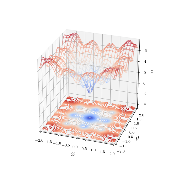
Rastrigin function
# Rastrigin function
Z = 10*2+(X**2-10*np.cos(2*np.pi*X))+(Y**2-10*np.cos(2*np.pi*Y))
$$f(\mathbf{x})=10 d+\displaystyle \sum_{i=1}^{d}\left[x_{i}^{2}-10 \cos \left(2 \pi x_{i}\right)\right]$$点 $\mathbf{x}^{*}=\left(0, \cdots, 0\right)$ で大域的最適解 $f\left(\mathbf{x}^{*}\right)=0$ をとる多峰性関数($d$は次元数)。
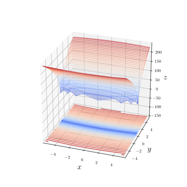
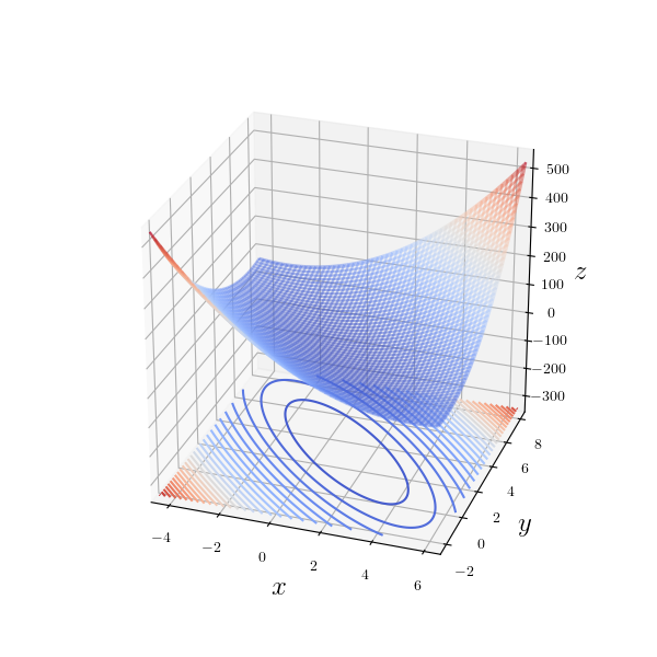
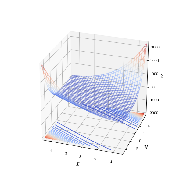
Rosenbrock function (banana function)
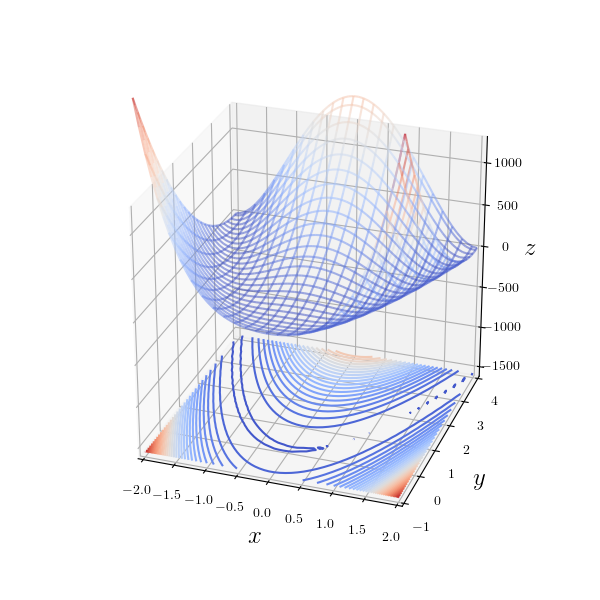
# Rosenbrock function (banana function)
Z = 100*(Y - X**2)**2 - (X - 1)**2
$$f(\mathbf{x})=\displaystyle \sum_{i=1}^{d-1}\left[100\left(x_{i+1}-x_{i}^{2}\right)^{2}+\left(x_{i}-1\right)^{2}\right]$$点 $\mathbf{x}^{*}=\left(1, \cdots, 1\right)$ で大域的最適解 $f\left(\mathbf{x}^{*}\right)=0$ をとる単峰性関数($d$は次元数)。大域的最適解が放物線状の狭い谷にあり、収束性を悪化させることで有名。その形状から別名「バナナ関数」とも呼ばれる。
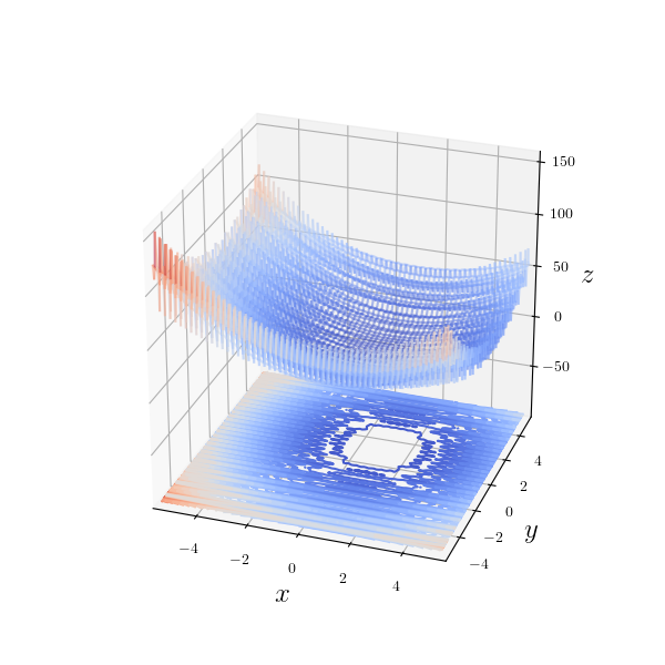
Sphere function
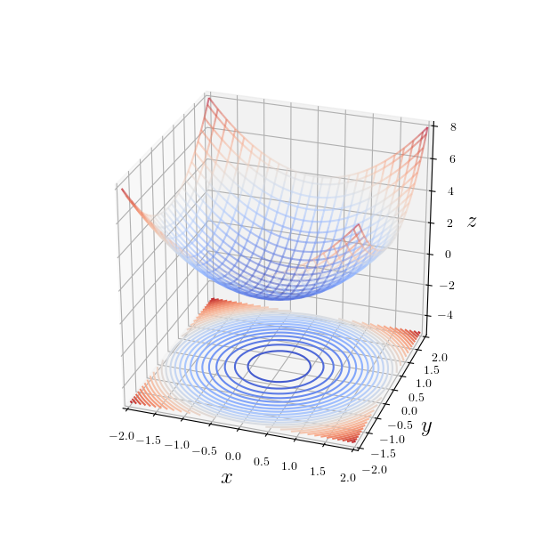
# Sphere function
Z = X**2 + Y**2
$$f(\mathbf{x})=\displaystyle \sum_{i=1}^{d}x_{i}^2$$点 $\mathbf{x}^{*}=\left(0, \cdots, 0\right)$ で大域的最適解 $f\left(\mathbf{x}^{*}\right)=0$ をとる単峰性関数($d$は次元数)。単純な(超)球面関数。
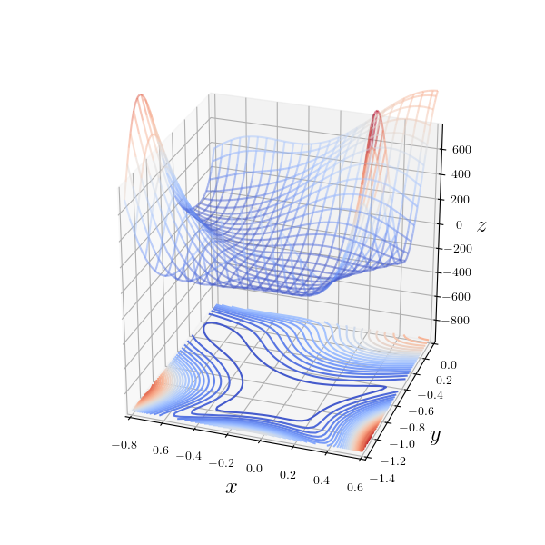
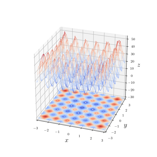
Shubert function
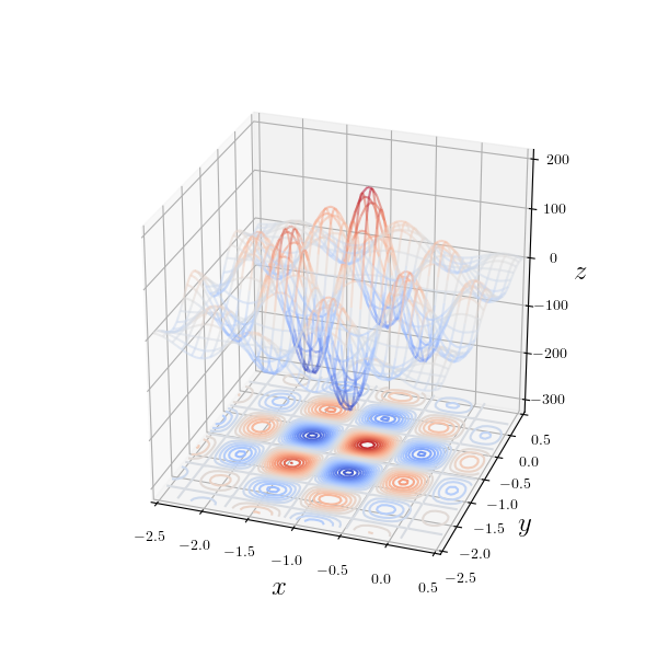
# Shubert function
f1 = (np.cos(1+(1+1)*X)+2*np.cos(2+(2+1)*X)+3*np.cos(3+(3+1)*X)+4*np.cos(4+(4+1)*X)+5*np.cos(5+(5+1)*X))
f2 = (np.cos(1+(1+1)*Y)+2*np.cos(2+(2+1)*Y)+3*np.cos(3+(3+1)*Y)+4*np.cos(4+(4+1)*Y)+5*np.cos(5+(5+1)*Y))
Z = f1 * f2
$$\small f(\mathbf{x})=\displaystyle \left(\sum_{i=1}^{5} i \cos \left((i+1) x_{1}+i\right)\right)\left(\sum_{i=1}^{5} i \cos \left((i+1) x_{2}+i\right)\right)$$点 $\mathbf{x}^{*}=\left( -0.80032… , -1.42512…\right)$ などで大域的最適解 $f\left(\mathbf{x}^{*}\right)=0$ をとる多峰性関数。大域的最適解を与える座標は周期的に存在する。
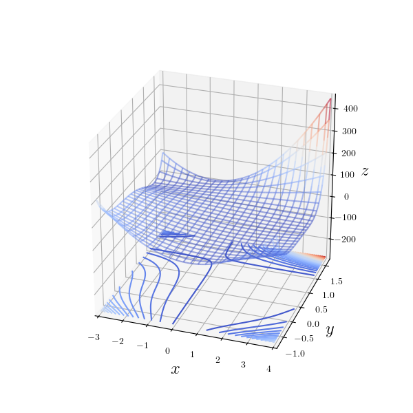
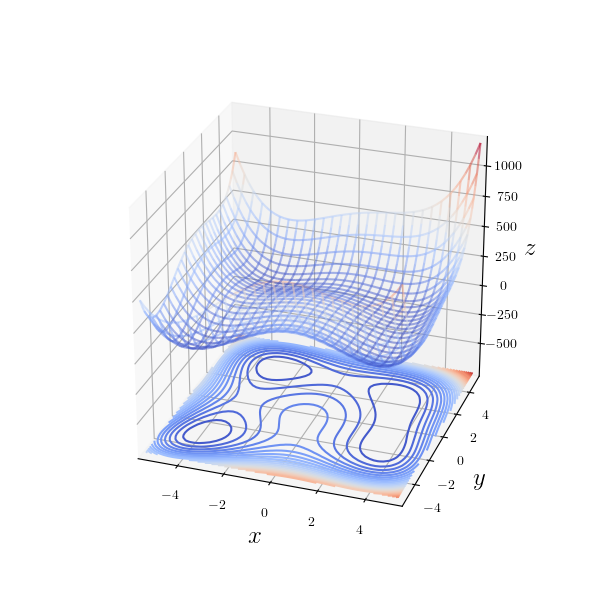
Styblinski-Tang function
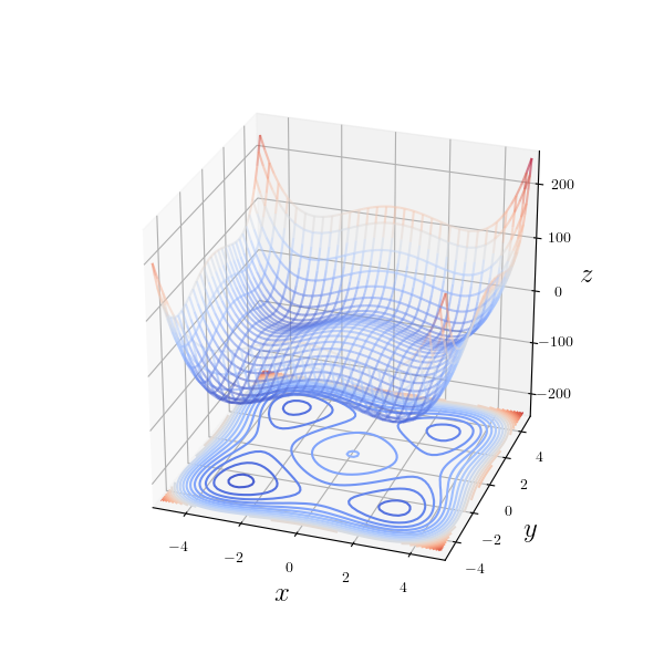
# Styblinski-Tang function
Z = 1/2 * ((X**4 - 16*X**2 + 5*X) + (Y**4 - 16*Y**2 + 5*Y))
$$f(\mathbf{x})=\dfrac{1}{2} \displaystyle \sum_{i=1}^{d}\left(x_{i}^{4}-16 x_{i}^{2}+5 x_{i}\right)$$点 $\mathbf{x}^{*}=\left( -2.90353… , \cdots ,\, -2.90353…\right)$ で大域的最適解 $f\left(\mathbf{x}^{*}\right)=-39.16616… \times d$ をとる多峰性関数($d$は次元数)。$d=2$ の場合は$( 2.74680…, -2.90353… )$、$( 2.74680… , 2.74680… )$、$( -2.90353… , 2.74680… )$で局所最適解をもつ。
Three-hump camel function
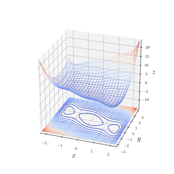
# Three-hump camel function
Z = 2*X**2 - 1.05*X**4 + X**6/6 + X*Y + Y**2
$$f(\mathbf{x})=2 x_{1}^{2}-1.05 x_{1}^{4}+\frac{x_{1}^{6}}{6}+x_{1} x_{2}+x_{2}^{2}$$点 $\mathbf{x}^{*}=\left(0,\, 0\right)$ で大域的最適解 $f\left(\mathbf{x}^{*}\right)=0$ をとる多峰性関数。名前の通り、曲面に窪みが3つ存在する。$( -1.74755… , 0.87377… )$、$( 1.74755… , -0.87377… )$で局所最適解をもつ。
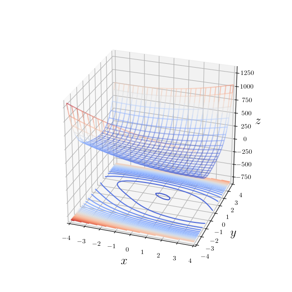
Zakharov function
# Zakharov function
Z = X**2+Y**2+(0.5*(X+2*Y))**2+(0.5*(X+2*Y))**4
$$f(\mathbf{x})= \displaystyle \sum_{i=1}^{d} x_{i}^{2}+\left(\sum_{i=1}^{d} 0.5 i x_{i}\right)^{2}+\left(\sum_{i=1}^{d} 0.5 i x_{i}\right)^{4}$$点 $\mathbf{x}^{*}=\left(0, \cdots \, 0\right)$ で大域的最適解 $f\left(\mathbf{x}^{*}\right)=0$ をとる単峰性関数($d$は次元数)。
リンク
ベンチマーク用の関数はこれ以外にも沢山あります。興味がある方のためにリンク(外部)を貼っておきます。
参考資料:
“Benchmark Functions“(benchmarkfcns)
“Optimization Test Problems“(Virtual Library of Simulation Experiments)
“Optimization & Eye Pleasure: 78 Benchmark Test Functions for Single Objective Optimization“(towards data science)
「最適化アルゴリズムを評価するベンチマーク関数まとめ」(Qiita)